Understanding the Spanning Tree Protocols

Choosing the Spanning Tree Protocols

The Spanning Tree algorithm works by designating a single switch (The Root Bridge) in the network as the root or the parent to all the switches, and then all the switches in the network will use the same algorithm to form a unique path that reaches all the way back to the Root Bridge from itself, with some switches establishing a blocking point (a port on a switch) somewhere along these paths if these paths form a loop. There are 3 versions of the Spanning Tree protocol, STP, RSTP, MSTP, and they are backward compatible.

The STP protocol

This is the original Spanning Tree protocol, and it has been superseded by both the RSTP and MSTP protocol. It is based on a network with a maximum diameter of no more than 17 switches. It uses timers to synchronize any changes in the network topology, and this could take minutes. It is not recommended that you use this version of the Spanning Tree protocol.

The RSTP protocol

The RSTP protocol is the new enhanced version of the original STP protocol. It uses an enhanced negotiation mechanism to directly synchronize topology changes between switches, it no longer uses timers as in the original STP protocol, which results in a much faster reconvergence time. The maximum allowed network diameter for the RSTP protocol is 40 switches.

The MSTP Protocol

The MSTP protocol extends the RSTP protocol by simultaneously running multiple instances of the Spanning Tree protocol and mapping different VLANs to each instance, thus providing load balance across multiple switches. The MSTP protocol accomplishes this by creating new extended sections within the RSTP protocol, called Regions, which runs a new Spanning Tree protocol. Within each Region, the MSTP protocol can accommodate a network diameter of up to 40 switches. There can be a maximum of 40 Regions in a single MSTP network.

The Root Bridge & Backup Root Bridge

To configure the Spanning Tree protocol on your network, you will need to set up a Root Bridge and, at least, one Backup Root Bridge. Although a Root Bridge will be automatically configured by the Spanning Tree protocol by default, it is better to manually configure a powerful high-end switch at the center of the network (this is often a layer 3 switch) as the designated Root Bridge. Because the Root Bridge will be the parent of all the switches in the Spanning Tree topology, the Root Bridge will usually receive the greatest share of the traffic load. By placing the Root Bridge at the center of the network you can also distribute the traffic to the network more efficiently. For the same reason as with the Root Bridge above, as well as for troubleshooting and diagnostic purposes, a Backup Root Bridge should also be configured on the network. This will ensure that a properly configured Backup Root Bridge will take over and become the Root Bridge for the network, in the event that the Root Bridge fails.

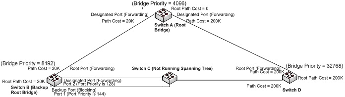
To configure a switch to be the Root Bridge of a Spanning Tree network, you must modify the Bridge ID of the switch to be the lowest among all the switches within the network. Each Spanning Tree switch must have a unique Bridge ID. This Bridge ID is a concatenation of 3 values: a 4 bit Bridge Priority (most significant), a 12 bit System ID (less significant), and the 48 bit MAC address of the local switch (least significant). To configure a switch to be the Root Bridge, you must make sure that the Bridge Priority (which is the most significant 4 bit of the Bridge ID) of the switch is the lowest among any of the switches on the network. Similarly for the Backup Root Bridge, it must have the next lowest Bridge Priority of all the switches. See below for an illustration.

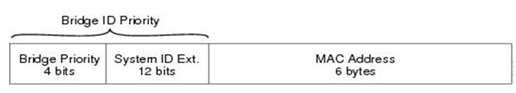
Bridge ID is a concatenation of 3 values: a 4 bit Bridge Priority (most significant), a 12 bit System ID (less significant), and the 48 bit MAC address of the local switch (least significant).

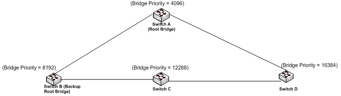
In the diagram above, switch A is the Root Bridge for entire the network because it has the lowest Bridge Priority value and switch B is the Backup Root Bridge for entire the network because it has the next lowest Bridge Priority value.

The Network Diameter

Another major consideration in implementing the Spanning Tree protocol on your network is the network diameter. In both the older STP and the newer RSTP protocol, there is a parameter called Max Age that should be adjusted according to the actual network diameter. The network diameter, in this case, is simply the total number of switches that belong to the longest daisy chain in the network which results when a link is broken in that daisy chain in the worst case scenario. In the older STP protocol, the Max Age parameter is calculated based on the network diameter minus one and the number of seconds that it might take to receive a BPDU. In the newer RSTP protocol, the Max Age parameter will be used simply as a hop count limit on how far the Spanning Tree protocol packet can propagate throughout the network topology, therefore, it must be configured with a value that is much greater than the network diameter. The Max Age parameters will need to be configured on the current Root Bridge only, therefore, it must be configured correctly on both the Root Bridge as well as on the Backup Bridge (in the event when the Root Bridge fails) to ensure that the Spanning Tree information can be propagated successfully from the Root Bridge (or the Backup Root Bridge, if the Root Bridge failed) to the furthest switch in the topology. The default value for the “Max Age” parameter is 20 (by default its value must be between 6 and 20).

Spanning Tree Port Roles

In a stable RSTP topology, each port on a switch can function in any one of 4 different Spanning Tree port roles. These Spanning Tree port roles are “Root Port”, “Designated Port”, “Alternate Port”, and “Backup Port”; and they are determined by two different types of comparison algorithms. They are further explained in the next 4 sections.

Root Port

Every Spanning Tree switch must have one and only one “Root Port” (excepting the Root Bridge). This is so that there will not be a switching loop in the network. The Root Port is the only port on a switch that has a direct path back to the Root Bridge, and if a switch were allowed to have more than one Root Port, then there will be multiple paths back to the Root Bridge from the local switch, this will cause switching loops in the network. The Root Port of a switch will be forwarding and receiving data packets for the local switch on the link that the port is connected to. The first type of comparison algorithm is used to determine the Root Port on a switch. The Root Port of a switch is determined by the local port with the lowest Root Path Cost for the switch unless there is a tie with another port, in which case it will be determined by the port with the lowest neighbor Bridge ID. If there is still a tie with the neighbor Bridge ID (as when a switch is connected to a neighbor bridge with more than one link), then the Root Port of the local switch will be determined by the local port with the lowest Port ID of the neighbor bridge in question. The Root Path Cost of a local port on a switch is determined by adding the Path Cost of the local port to the Root Path Cost of the neighbor bridge on the link that the local port is connected to. By default, each port on a Spanning Tree switch will be assigned a Path Cost based on the port's transmission speed, according to the IEEE standard below.

Link speed	Recommended value
Less than or equal 100Kb/s	200,000,000
1 Mb/s	20,000,000
10 Mb/s	2,000,000
100 Mb/s	200,000
1 Gb/s	20,000
10 Gb/s	2,000
100 Gb/s	200
1 Tb/s	20
10 Tb/s	2

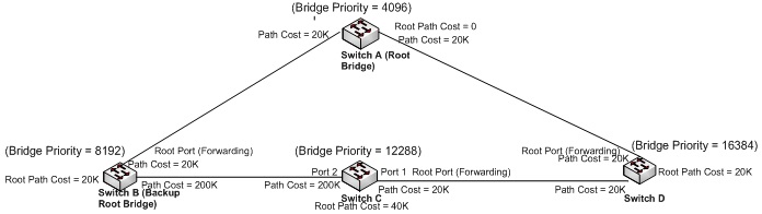
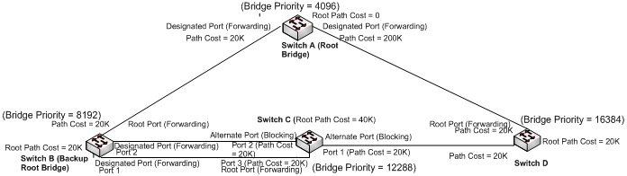
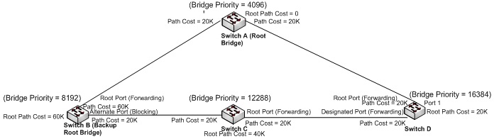
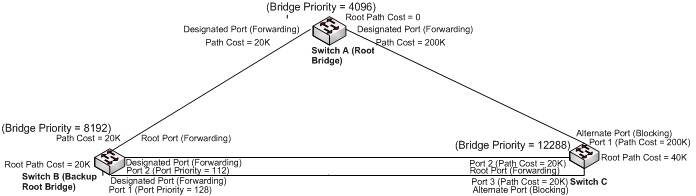
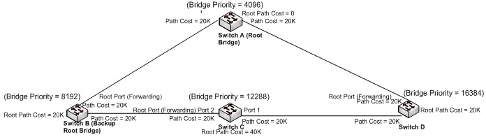
The first type of comparison algorithm is used to determine the Root Port on a switch. The Root Port of a switch is determined by the local port with the lowest Root Path Cost for the switch unless there is a tie with another port. In the diagram above, all 3 ports on switch Chas the same Root Path Cost, and two of the ports (1 and 2) has the same neighbor bridge ID (4096 + Mac), which is superior to the neighbor bridge ID of port 3 (8192 + Mac). Since both ports 1 and 2 on switch C receives identical neighbor bridge information, switch C will have to use the Port ID of the local switch port to break the tie. In this case, port 1 will become the Root Port on switch C.

Designated Port

On a link between any two Spanning Tree Bridges, if both bridges have Root Ports that are not connected to this link, then there can only be one port belonging to only one switch that is connected to this link through which data packets can be allowed to be forwarded back to the Root Bridge. This is so that there will not be a switching loop in the network. This port is the Designated Port on a local switch on that link, and this local switch will be the Designated Bridge on that link. A switch can have more than one Designated Port connecting to the same or to a different switch. The second type of comparison algorithm is used to determine the Designated Port on a switch. The Designated Port of a switch on a link is determined by a comparison of the Root Path Cost between the local switch and the neighboring switch on that link; whichever switch that has the lowest Root Path Cost will be considered the Designated Bridge with the Designated Port on that link, and the privilege to forward traffic from that link back to the Root Bridge. If there is a tie between the Root Path Cost of the local switch and the neighboring switch, then the Bridge ID of the switches will be used to break the tie; whichever switch with the lower Bridge ID will be the switch with the Designated Port on that link.

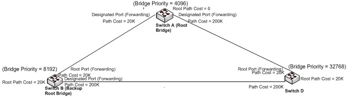
The second type of comparison algorithm is used to determine the Designated Port on a switch. The Designated Port of a switch on a link is determined by a comparison of the Root Path Cost between the local switch and the neighboring switch on that link. In the diagram above, switch B has the superior Root Path Cost on the link between switch B and switch D, therefore, switch B is the Designated Bridge on this link and the port on switch B that connects to this link is the Designated Port on switch B for this link.

The second type of comparison algorithm is used to determine the Designated Port on a switch. The Designated Port of a switch on a link is determined by a comparison of the Root Path Cost between the local switch and the neighboring switch on that link. In the diagram above, both switch B and switch D has the same Root Path Cost (20K) on the link between them, therefore, the Bridge ID of both switches are used to determine which switch will have the Designated Port. Since switch B has the superior Bridge ID between the two, switch B will be the Designated Bridge on this link and the port on switch B that connects to this link will be the Designated Port on switch B for this link.

Alternate Port

If the application of the second type of comparison algorithm has determined that a port on a local switch is not the Designated Port on that switch for a particular link (i.e. the local switch has a higher Root Path Cost or higher Bridge ID, in the case where the Root Path Cost is the same between two switches than the neighboring switch on that link), then this port should become the Alternated Port on the local switch. This means that the local switch now has an alternate path (through the Designated Port of the neighboring switch on that link) that can lead back directly to the Root Bridge, which is in addition to the existing path through the Root Port of the local switch. Since multiple paths leading back to the Root Bridge from a local switch will form switching loops in the network, all Alternated Ports formed this way on a local switch will not be allowed to forward or to receive any data packets on the link that the Alternate Port is connected to.

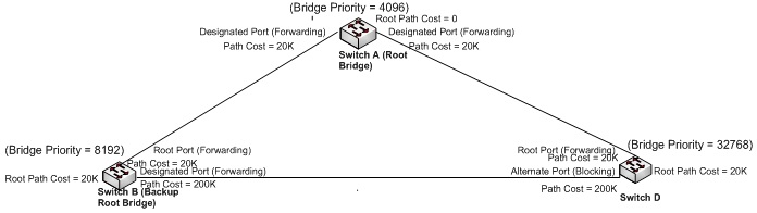
The second type of comparison algorithm is also used to determine the Alternate Port on a switch. In the diagram above, the Root Path Cost for switch D is not superior to the Root Path Cost for switch B on the link between them, therefore, switch B is the Designated Bridge on this link, and since the Root Port for switch D is not on this link, the port on switch D that connects to this link will have to become the Alternate Port on switch B for this link.

If the application of the second type of comparison algorithm has produced a tie among the Root Path Costs between the two switches on a link, then the lowest Bridge ID among the two switches will be used to break the tie. In the diagram above, both switch B and switch D has the same Root Path Cost (20K) on the link between them, therefore, the Bridge ID of both switches are used to determine which switch will have the Designated Port. Since switch B has the superior Bridge ID between the two, switch B will be the Designated Bridge on this link, and since the Root Port for switch D is not on this link, the port on switch D that connects to this link will have to become the Alternate Port on switch B for this link.

Backup Port

Sometimes it will happen that a port will be accidentally linked up to another port on the same local switch. When this happens on a switch, both the Root Path Cost and the Bridge ID used in the second type of comparison algorithm will be the same, in this case, the Port ID on the local switch will be used to break the tie; the port with the lowest Port ID on the local switch will be the Designated Port, and the other port will be the Backup Port.

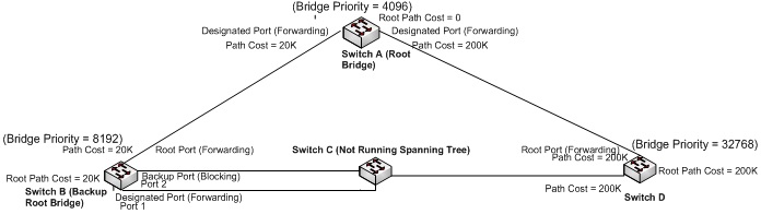
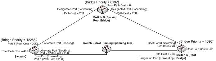
In the above diagram, Switch C is not running any Spanning Tree protocol, which means it will flood all received Spanning Tree information out to all the connected neighbor bridges (including switch B itself). This means that the Spanning Tree information sent from Switch B will be processed directly by Switch D and Switch B itself (it will receive the same Spanning Tree packet on port 2 which was sent out from port 1, and vice versa). For switch B, since both the Root Path Cost and the Bridge ID in the Spanning Tree packets received on ports 1 & 2 will be same (they came from the same switch, namely, switch B itself), in this case, the Port ID in the Spanning Tree packet will be used to break the tie. Since port 1 on switch B received a Spanning Tree packet with a port ID that is inferior to itself (port 2, which is inferior to port 1), port 1 becomes the Designated Port, and port 2 will become the Backup Port.

Path Cost

By default, each port on a Spanning Tree switch will be assigned a Path Cost based on the port's transmission speed, according to the IEEE standard below.

Link speed	Recommended value
Less than or equal 100Kb/s	200,000,000
1 Mb/s	20,000,000
10 Mb/s	2,000,000
100 Mb/s	200,000
1 Gb/s	20,000
10 Gb/s	2,000
100 Gb/s	200
1 Tb/s	20
10 Tb/s	2

Although you will rarely need to adjust these settings because the default values should work fine in most scenarios, however, there are times when you might need to adjust these values manually, in order to influence the location of the Alternate Port or the Root Port.

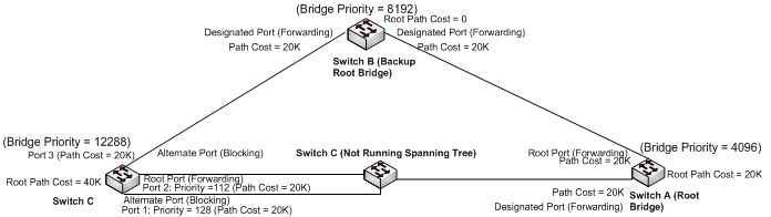
In the above RSTP network with a redundant ring, the blocking port for the redundant ring is located on Switch B, based on the Bridge ID of the Root Bridge.

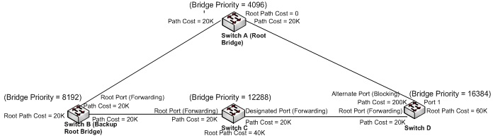
After modifying the Path Cost of port 1 on Switch D from 20K to 200K, this port has now become the blocking port for the redundant ring.

Port Priority

By default each port on a Spanning Tree switch will be assigned a Port Priority of 128, according to the IEEE standard. This Port Priority is part of the Port ID, which is a concatenation of 2 values: Port Priority (4 bits) + Interface ID (12 bits). Although you will rarely need to adjust these settings because the default values should work fine in most scenarios, however, there are times when you might need to adjust these values manually, in order to influence the location of the Alternate Port or the Root Port or the Backup Port.

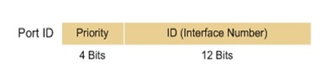
Port Priority is part of the Port ID, which is a concatenation of 2 values: Port Priority (4 bits) + Interface ID (12 bits).

In the above diagram, Switch C is not running any Spanning Tree protocol, which means it will flood all received Spanning Tree information out to all the connected neighbor bridges (including switch B itself). This means that the Spanning Tree information sent from Switch B will be processed directly by Switch D and Switch B itself (it will receive the same Spanning Tree packet on port 2 which was sent out from port 1, and vice versa). For switch B, since both the Root Path Cost and the Bridge ID in the Spanning Tree packets received on ports 1 & 2 will be same (they came from the same switch, namely, switch B itself), in this case, the Port ID in the Spanning Tree packet will be used to break the tie. Even though port 1 is superior to port 2 in Interface ID, but port 1 has an inferior Port Priority (144) then port 2 (128), and since Port Priority is the more significant portion of the Port ID than Interface ID when Port ID is considered as a whole, in this case, the Port ID of Port 1 is actually inferior to the Port ID of port 2. Because port 1 on switch B received a Spanning Tree packet with a Port ID that is superior to itself, port 1 will become the Backup Port, and port 2 will become the Designated Port.

The first type of comparison algorithm is used to determine the Root Port on a switch. The Root Port of a switch is determined by the local port with the lowest Root Path Cost for the switch unless there is a tie with another port. In the diagram above, both ports 2 and 3 have the same Root Path Cost (40K), which is superior to port 1 (200K), and both ports have the same neighbor bridge ID (8192 + Mac) but with different neighbor bridge Port ID. Normally, port 3 should become the Root Port on switch C because its neighbor bridge interface ID (neighbor bridge interface # 1) is superior to port 2 (neighbor bridge interface # 2), however, since the neighbor bridge Priority ID of port 2 (112) is superior to the neighbor bridge Priority ID of port 3 (128), in this case, port 2 will become the Root Port on switch C.

The first type of comparison algorithm is used to determine the Root Port on a switch. The Root Port of a switch is determined by the local port with the lowest Root Path Cost for the switch unless there is a tie with another port. In the diagram above, all 3 ports on switch Chas the same Root Path Cost, and two of the ports (1 and 2) has the same neighbor bridge ID (4096 + Mac), which is superior to the neighbor bridge ID of port 3 (8192 + Mac). Since both ports 1 and 2 on switch C receives identical neighbor bridge information, switch C will have to use the Port ID of the local switch port to break the tie. In a normal scenario, port 1 should become the Root Port on switch C because its interface ID is superior to port 2 on the local switch, but because the Priority ID of the local switch port 2 (112) is superior to the Priority ID of the local switch port 1 (128), in this case, port 2 will become the Root Port on switch C.

Point to Point Link

The purpose of this feature of the RSTP protocol is to be backward compatible with the older STP protocol. Unlike the original STP protocol, the RSTP protocol does not use timers to synchronize changes in the Spanning Tree topology; instead, it uses a direct negotiation process with the neighboring switches to quickly synchronize any changes in the Spanning Tree topology. In order for this fast negotiation process to work well, there can only be two switches on the same link, and there cannot be any switches running the older STP protocol. The RSTP protocol will by default assume any full-duplex link as a “Point to Point Link”, which means that it will assume the only other neighbor switch on this link is running the RSTP protocol, but if the switch should detect that the neighbor switch is not running the RSTP protocol, it will assume the port to be a “Shared” port, which means that there could be switches running the older STP protocol on this link.

Edge Port

Next, you may need to adjust the “Edge Port” settings according to your network environment. By default, the RSTP protocol will treat each port as an RSTP port which can potentially connect to another neighbor switch, and as such the switch will react to a linkup event on a port by sending out a Topology Change notification to the neighbor bridges, this will cause both the local switch and neighbor switches to erase their MAC tables (the table containing the Device ID to port mappings), and start anew to relearn the Device ID to port mappings. This process will cause momentary traffic flooding on the network while the switch has not as yet learned the destination ports that the switch should forward the received packets to. You can avert this process when it is not necessarily by using the “Edge Port” feature.